DL Project 2 MNIST Digit classification using NN
Deep learning එකේ "hello world" එකයි — අත් අකුරෙන් ලියපු ඉලක්කම් හඳුනාගැනීම — මොකද ඉක්මනට train කරන්න තරම් සරලයි, ඒත් core neural-network concept ඔක්කොම උගන්වන්න තරම් real.
The "hello world" of deep learning — recognizing handwritten digits — because it's simple enough to train fast, yet real enough to teach every core neural-network concept.
Lesson 63 of 64 · Part 5 · Shipping Models to the World · DL 3. MNIST Digit Classification · bilingual notes (English + සිංහල)
Why this matters. The "hello world" of deep learning — recognizing handwritten digits — because it's simple enough to train fast, yet real enough to teach every core neural-network concept.
සිංහලෙන්: Deep learning එකේ "hello world" එකයි — අත් අකුරෙන් ලියපු ඉලක්කම් හඳුනාගැනීම — මොකද ඉක්මනට train කරන්න තරම් සරලයි, ඒත් core neural-network concept ඔක්කොම උගන්වන්න තරම් real.
What you'll use this for. The same core architecture used here — a neural network reading pixel grids — scales up, with more layers and tricks, into the exact image classifiers used in real apps.
සිංහලෙන්: මෙතන පාවිච්චි කරන එකම core architecture එක — pixel grids කියවන neural network එකක් — layers සහ tricks වැඩිය කරලා, real apps වල පාවිච්චි කරන image classifiers හරියටම ඒම විදිහටම scale වෙනවා.
Key principles
- Flattening turns a 2D image into a 1D list a basic neural network can read. A 28×28 pixel digit becomes a single row of 784 numbers before it enters the network — the spatial layout is temporarily lost, which is exactly the limitation CNNs later fix.
Flatten කිරීමෙන් 2D image එකක්, basic neural network එකකට කියවන්න පුළුවන් 1D list එකක් බවට හරවනවා
Walkthrough
MNIST Handwritten Digit Clasification using Deep Learning (Neural Network)
Importing the Dependencies
import numpy as np
import matplotlib.pyplot as plt
import seaborn as sns
import cv2
from google.colab.patches import cv2_imshow
from PIL import Image
import tensorflow as tf
tf.random.set_seed(3)
from tensorflow import keras
from keras.datasets import mnist
from tensorflow.math import confusion_matrix
Loading the MNIST data from keras.datasets
(X_train, Y_train), (X_test, Y_test) = mnist.load_data()Output
Downloading data from https://storage.googleapis.com/tensorflow/tf-keras-datasets/mnist.npz
11493376/11490434 [==============================] - 0s 0us/step
11501568/11490434 [==============================] - 0s 0us/steptype(X_train)Output
numpy.ndarray# shape of the numpy arrays
print(X_train.shape, Y_train.shape, X_test.shape, Y_test.shape)Output
(60000, 28, 28) (60000,) (10000, 28, 28) (10000,)Training data = 60,000 Images
Test data = 10,000 Images
Image dimension --> 28 x 28
Grayscale Image --> 1 channel
# printing the 10th image

print(X_train[10])
Output
[[  0   0   0   0   0   0   0   0   0   0   0   0   0   0   0   0   0   0
    0   0   0   0   0   0   0   0   0   0]
 [  0   0   0   0   0   0   0   0   0   0   0   0   0   0   0   0   0   0
    0   0   0   0   0   0   0   0   0   0]
 [  0   0   0   0   0   0   0   0   0   0   0   0   0   0   0   0   0   0
    0   0   0   0   0   0   0   0   0   0]
 [  0   0   0   0   0   0   0   0   0   0   0   0   0   0   0   0   0   0
    0   0   0   0   0   0   0   0   0   0]
 [  0   0   0   0   0   0   0   0   0   0   0  42 118 219 166 118 118   6
    0   0   0   0   0   0   0   0   0   0]
 [  0   0   0   0   0   0   0   0   0   0 103 242 254 254 254 254 254  66
    0   0   0   0   0   0   0   0   0   0]
 [  0   0   0   0   0   0   0   0   0   0  18 232 254 254 254 254 254 238
   70   0   0   0   0   0   0   0   0   0]
 [  0   0   0   0   0   0   0   0   0   0   0 104 244 254 224 254 254 254
  141   0   0   0   0   0   0   0   0   0]
 [  0   0   0   0   0   0   0   0   0   0   0   0 207 254 210 254 254 254
   34   0   0   0   0   0   0   0   0   0]
… (38 more lines)print(X_train[10].shape)Output
(28, 28)# displaying the image
plt.imshow(X_train[25])
plt.show()
# print the corresponding label
print(Y_train[25])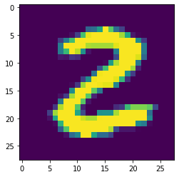
Output
2Image Lables
print(Y_train.shape, Y_test.shape)Output
(60000,) (10000,)# unique values in Y_train
print(np.unique(Y_train))
# unique values in Y_test
print(np.unique(Y_test))Output
[0 1 2 3 4 5 6 7 8 9]
[0 1 2 3 4 5 6 7 8 9]
We can use these labels as such or we can also apply One Hot Encoding
All the images have the same dimensions in this dataset, If not, we have to resize all the images to a common dimension
# scaling the values

X_train = X_train/255
X_test = X_test/255# printing the 10th image
print(X_train[10])Output
[[0.         0.         0.         0.         0.         0.
  0.         0.         0.         0.         0.         0.
  0.         0.         0.         0.         0.         0.
  0.         0.         0.         0.         0.         0.
  0.         0.         0.         0.        ]
 [0.         0.         0.         0.         0.         0.
  0.         0.         0.         0.         0.         0.
  0.         0.         0.         0.         0.         0.
  0.         0.         0.         0.         0.         0.
  0.         0.         0.         0.        ]
 [0.         0.         0.         0.         0.         0.
  0.         0.         0.         0.         0.         0.
  0.         0.         0.         0.         0.         0.
  0.         0.         0.         0.         0.         0.
  0.         0.         0.         0.        ]
 [0.         0.         0.         0.         0.         0.
  0.         0.         0.         0.         0.         0.
  0.         0.         0.         0.         0.         0.
… (122 more lines)
Building the Neural Network
# setting up the layers of the Neural  Network

model = keras.Sequential([
                          keras.layers.Flatten(input_shape=(28,28)),
                          keras.layers.Dense(50, activation='relu'),
                          keras.layers.Dense(50, activation='relu'),
                          keras.layers.Dense(10, activation='sigmoid')
])# compiling the Neural Network
model.compile(optimizer='adam',
loss = 'sparse_categorical_crossentropy',
metrics=['accuracy'])# training the Neural Network
model.fit(X_train, Y_train, epochs=10)Output
Epoch 1/10
1875/1875 [==============================] - 5s 2ms/step - loss: 0.2983 - accuracy: 0.9138
Epoch 2/10
1875/1875 [==============================] - 4s 2ms/step - loss: 0.1368 - accuracy: 0.9591
Epoch 3/10
1875/1875 [==============================] - 4s 2ms/step - loss: 0.1025 - accuracy: 0.9682
Epoch 4/10
1875/1875 [==============================] - 4s 2ms/step - loss: 0.0835 - accuracy: 0.9744
Epoch 5/10
1875/1875 [==============================] - 4s 2ms/step - loss: 0.0685 - accuracy: 0.9787
Epoch 6/10
1875/1875 [==============================] - 4s 2ms/step - loss: 0.0609 - accuracy: 0.9806
Epoch 7/10
1875/1875 [==============================] - 4s 2ms/step - loss: 0.0513 - accuracy: 0.9838
Epoch 8/10
1875/1875 [==============================] - 4s 2ms/step - loss: 0.0458 - accuracy: 0.9855
Epoch 9/10
1875/1875 [==============================] - 4s 2ms/step - loss: 0.0402 - accuracy: 0.9873
… (2 more lines)
Output
<keras.callbacks.History at 0x7f5aea3f8850>Training data accuracy = 98.9%
Accuracy on Test data:
loss, accuracy = model.evaluate(X_test, Y_test)
print(accuracy)
Output
313/313 [==============================] - 1s 2ms/step - loss: 0.1040 - accuracy: 0.9710
0.9710000157356262
Test data accuracy = 97.1%
print(X_test.shape)Output
(10000, 28, 28)# first data point in X_test
plt.imshow(X_test[0])
plt.show()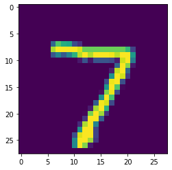
print(Y_test[0])Output
7Y_pred = model.predict(X_test)print(Y_pred.shape)Output
(10000, 10)print(Y_pred[0])Output
[3.5130084e-03 6.7106444e-01 6.6638464e-01 8.5868883e-01 6.2501094e-05
 9.0813637e-04 4.0907306e-08 9.9999774e-01 1.3417095e-02 6.5949798e-02]
model.predict() gives the prediction probability of each class for that data point
# converting the prediction probabilities to class label

label_for_first_test_image = np.argmax(Y_pred[0])
print(label_for_first_test_image)
Output
7# converting the prediction probabilities to class label for all test data points
Y_pred_labels = [np.argmax(i) for i in Y_pred]
print(Y_pred_labels)Output
[7, 2, 1, 0, 4, 1, 4, 9, 6, 9, 0, 6, 9, 0, 1, 5, 9, 7, 3, 4, 9, 6, 6, 5, 4, 0, 7, 4, 0, 1, 3, 1, 3, 4, 7, 2, 7, 1, 2, 1, 1, 7, 4, 2, 3, 5, 1, 2, 4, 4, 6, 3, 5, Y_test --> True labels
Y_pred_labels --> Predicted Labels
Confusin Matrix
conf_mat = confusion_matrix(Y_test, Y_pred_labels)print(conf_mat)Output
tf.Tensor(
[[ 969    1    1    0    1    1    2    2    3    0]
 [   0 1122    1    2    0    4    2    0    4    0]
 [   5    0  999    1    7    1    2    6   11    0]
 [   0    0    5  966    0   23    0    3    7    6]
 [   0    0    2    0  968    1    4    2    1    4]
 [   2    0    0    4    2  878    4    1    1    0]
 [   6    1    0    0    8   11  929    0    3    0]
 [   1    5    9    0    5    0    0  994    8    6]
 [   2    0    3    6    6   10    2    2  943    0]
[ 3 4 0 8 24 10 1 7 10 942]], shape=(10, 10), dtype=int32)plt.figure(figsize=(15,7))
sns.heatmap(conf_mat, annot=True, fmt='d', cmap='Blues')
plt.ylabel('True Labels')
plt.xlabel('Predicted Labels')Output
Text(0.5, 42.0, 'Predicted Labels')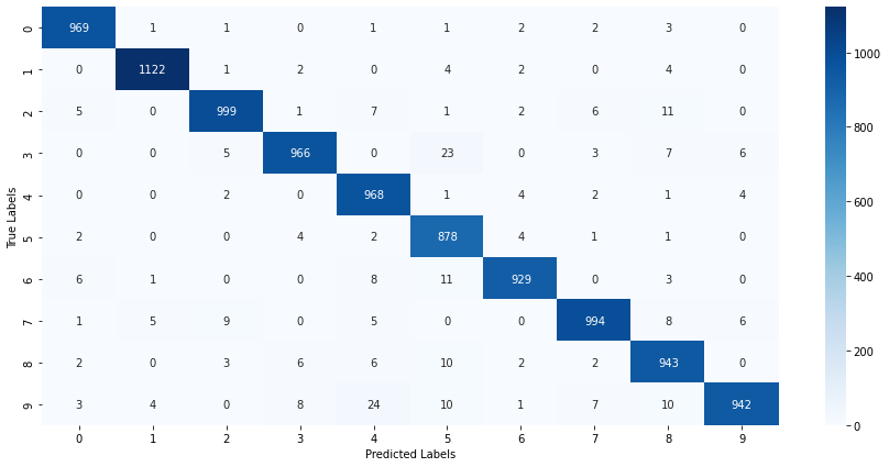
Building a Predictive System
input_image_path = '/content/MNIST_digit.png'

input_image = cv2.imread(input_image_path)type(input_image)Output
numpy.ndarrayprint(input_image)cv2_imshow(input_image)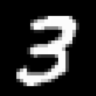
input_image.shapeOutput
(318, 318, 3)grayscale = cv2.cvtColor(input_image, cv2.COLOR_RGB2GRAY)grayscale.shapeOutput
(318, 318)input_image_resize = cv2.resize(grayscale, (28, 28))input_image_resize.shapeOutput
(28, 28)cv2_imshow(input_image_resize)
input_image_resize = input_image_resize/255type(input_image_resize)Output
numpy.ndarrayimage_reshaped = np.reshape(input_image_resize, [1,28,28])input_prediction = model.predict(image_reshaped)
print(input_prediction)Output
[[5.9389083e-10 9.4131142e-02 1.9494593e-03 1.0000000e+00 4.7541544e-08
6.3185507e-01 2.8182675e-13 2.7394295e-04 9.5208365e-01 4.5282638e-01]]input_pred_label = np.argmax(input_prediction)print(input_pred_label)Output
3Predictive System
input_image_path = input('Path of the image to be predicted: ')

input_image = cv2.imread(input_image_path)

cv2_imshow(input_image)

grayscale = cv2.cvtColor(input_image, cv2.COLOR_RGB2GRAY)

input_image_resize = cv2.resize(grayscale, (28, 28))

input_image_resize = input_image_resize/255

image_reshaped = np.reshape(input_image_resize, [1,28,28])

input_prediction = model.predict(image_reshaped)

input_pred_label = np.argmax(input_prediction)

print('The Handwritten Digit is recognised as ', input_pred_label)
Output
Path of the image to be predicted: /content/MNIST_digit.png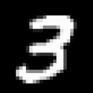
Output
The Handwritten Digit is recognised as 3Keep going: ← Lesson 62 · Lesson 64 → · Track it in the Self Guide
Finished this one?
Part of Self Guide · Stage 17: ML 5 — Shipping Models to the World. Progress is saved in this browser.