Implementing Linear Regression from scratch in Python
කලින් පාඩමේ theory එක, real numbers එක්ක test කරන්න පුළුවන් run වෙන code එකක් බවට හැරෙන්නෙ මෙතන.
This is where the theory from the previous lesson becomes running code you can actually test against real numbers.
Lesson 33 of 64 · Part 3 · Building Models from Scratch · Algorithms from Scratch · bilingual notes (English + සිංහල)
Why this matters. This is where the theory from the previous lesson becomes running code you can actually test against real numbers.
සිංහලෙන්: කලින් පාඩමේ theory එක, real numbers එක්ක test කරන්න පුළුවන් run වෙන code එකක් බවට හැරෙන්නෙ මෙතන.
What you'll use this for. Once this works on toy data, the exact same code structure is what powers sklearn.linear_model.LinearRegression internally.
සිංහලෙන්: Toy data එකකට මේක වැඩ කලාට පස්සෙ, ඒම code structure එකෙන්ම තමයි sklearn.linear_model.LinearRegression ඇතුළතින් වැඩ කරන්නෙ.
Key principles
- Testing on data you already know the answer for is how you verify the maths. If your from-scratch model can't recover a simple, known relationship (like y = 2x + 3), the bug is in your code, not your understanding of the concept.
දැනටමත් උත්තරය දන්න data එකකට test කිරීමෙන් තමයි maths එක verify කරන්නෙ
Walkthrough
Linear Regression:
Y = wX + b
Y --> Dependent Variable
X --> Independent Variable
w --> weight
b --> bias
Gradient Descent:
Gradient Descent is an optimization algorithm used for minimizing the loss function in various machine learning algorithms. It is used for updating the parameters of the learning model.
w = w - α*dw
b = b - α*db
Importing the Dependencies
# Importing numpy library
import numpy as np
Linear Regression
class Linear_Regression():

   def __init__( self, learning_rate, no_of_iterations ) :

        self.learning_rate = learning_rate

        self.no_of_iterations = no_of_iterations

    # fit function to train the model

   def fit( self, X, Y ) :

        # no_of_training_examples, no_of_features

        self.m, self.n = X.shape

        # initiating the weight and bias

        self.w = np.zeros( self.n )

        self.b = 0

        self.X = X

        self.Y = Y

        # implementing Gradient Descent for Optimization

        for i in range( self.no_of_iterations ) :

            self.update_weights()


    # function to update weights in gradient descent

   def update_weights( self ) :

        Y_prediction = self.predict( self.X )

        # calculate gradients

        dw = - ( 2 * ( self.X.T ).dot( self.Y - Y_prediction )  ) / self.m

        db = - 2 * np.sum( self.Y - Y_prediction ) / self.m

        # updating the weights

        self.w = self.w - self.learning_rate * dw

        self.b = self.b - self.learning_rate * db


    # Line function for prediction:

   def predict( self, X ) :

        return X.dot( self.w ) + self.b
Using Linear Regression model for Prediction
# importing the dependencies
import pandas as pd
from sklearn.model_selection import train_test_split
import matplotlib.pyplot as plt
Data Pre-Processing
# loading the data from csv file to a pandas dataframe

salary_data = pd.read_csv('/content/salary_data.csv')# printing the first 5 columns of the dataframe
salary_data.head()| YearsExperience | Salary | |
|---|---|---|
| 0 | 1.1 | 39343 |
| 1 | 1.3 | 46205 |
| 2 | 1.5 | 37731 |
| 3 | 2.0 | 43525 |
| 4 | 2.2 | 39891 |
# last 5 rows of the dataframe
salary_data.tail()| YearsExperience | Salary | |
|---|---|---|
| 25 | 9.0 | 105582 |
| 26 | 9.5 | 116969 |
| 27 | 9.6 | 112635 |
| 28 | 10.3 | 122391 |
| 29 | 10.5 | 121872 |
# number of rows & columns in the dataframe
salary_data.shape
Output
(30, 2)# checking for missing values
salary_data.isnull().sum()Output
YearsExperience    0
Salary             0
dtype: int64
Splitting the feature & target
X = salary_data.iloc[:,:-1].values
Y = salary_data.iloc[:,1].valuesprint(X)Output
[[ 1.1]
 [ 1.3]
 [ 1.5]
 [ 2. ]
 [ 2.2]
 [ 2.9]
 [ 3. ]
 [ 3.2]
 [ 3.2]
 [ 3.7]
 [ 3.9]
 [ 4. ]
 [ 4. ]
 [ 4.1]
 [ 4.5]
 [ 4.9]
 [ 5.1]
 [ 5.3]
… (12 more lines)print(Y)Output
[ 39343  46205  37731  43525  39891  56642  60150  54445  64445  57189
  63218  55794  56957  57081  61111  67938  66029  83088  81363  93940
  91738  98273 101302 113812 109431 105582 116969 112635 122391 121872]
Splitting the dataset into training & test data
X_train, X_test, Y_train, Y_test = train_test_split(X, Y, test_size=0.33, random_state = 2)Training the Linear Regression model
model = Linear_Regression(learning_rate = 0.02, no_of_iterations=1000)model.fit(X_train, Y_train)# printing the parameter values ( weights & bias)
print('weight = ', model.w[0])
print('bias = ', model.b)Output
weight =  9514.400999035135
bias =  23697.406507136307
y = 9514(x) + 23697
salary = 9514(experience) + 23697
Predict the salary value for test data
test_data_prediction = model.predict(X_test)print(test_data_prediction)Output
[ 36066.12780588  34163.24760607  66512.21100279  58900.69020357
  91249.65360029  80783.81250135 101715.49469922  52240.60950424
  42726.20850521  88395.33330058]
Visualizing the predicted values & actual Values
plt.scatter(X_test, Y_test, color = 'red')
plt.plot(X_test, test_data_prediction, color='blue')
plt.xlabel(' Work Experience')
plt.ylabel('Salary')
plt.title(' Salary vs Experience')
plt.show()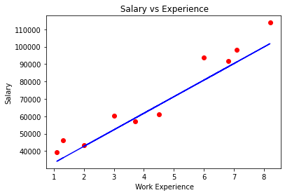
Keep going: ← Lesson 32 · Lesson 34 → · Track it in the Self Guide
Finished this one?
Part of Self Guide · Stage 15: ML 3 — Building Models from Scratch. Progress is saved in this browser.