Project 12 Big Mart Sales Prediction

අවුල් සහගත, සැබෑ retail data එකක regression project එකක් — missing values, mixed types, outliers — Parts 1 සිට 4 දක්වා ඉගෙන ගත්ත ඔක්කොම මුල්වතාවට එකට apply වෙන්නෙ මෙතන.

A regression project on messy, real retail data — missing values, mixed types, outliers — where everything from Parts 1 through 4 gets applied together for the first time.

17 May 20267 min readSelf Guide · Stage 16#Evaluating & Choosing Models#Hands-on Projects#Machine learning

Lesson 48 of 64 · Part 4 · Evaluating & Choosing Models · Hands-on Projects · bilingual notes (English + සිංහල)

Why this matters. A regression project on messy, real retail data — missing values, mixed types, outliers — where everything from Parts 1 through 4 gets applied together for the first time.

සිංහලෙන්: අවුල් සහගත, සැබෑ retail data එකක regression project එකක් — missing values, mixed types, outliers — Parts 1 සිට 4 දක්වා ඉගෙන ගත්ත ඔක්කොම මුල්වතාවට එකට apply වෙන්නෙ මෙතන.

What you'll use this for. Retailers use exactly this kind of model to forecast demand per store, per product — directly informing stocking and staffing decisions.

සිංහලෙන්: Store එකකට, product එකකට demand forecast කරන්න retailers පාවිච්චි කරන්නෙ හරියටම මේ වගේ model එකක් — stocking සහ staffing decisions වලට කෙලින්ම බලපානවා.

Key principles

Feature engineering often matters more than the choice of algorithm. Creating a smart feature (like "years since establishment" from a raw year column) frequently improves accuracy more than switching from one algorithm to another.
Feature engineering, algorithm එක තෝරගැනීමට වඩා ගොඩක් වෙලාවට වැදගත්

Walkthrough

Importing the Dependencies

ExamplePython

import numpy as np
import pandas as pd
import matplotlib.pyplot as plt
import seaborn as sns
from sklearn.preprocessing import LabelEncoder
from sklearn.model_selection import train_test_split
from xgboost import XGBRegressor
from sklearn import metrics

Data Collection and Processing

ExamplePython

# loading the data from csv file to Pandas DataFrame
big_mart_data = pd.read_csv('/content/Train.csv')

ExamplePython

# first 5 rows of the dataframe
big_mart_data.head()

	Item_Identifier	Item_Weight	Item_Fat_Content	Item_Visibility	Item_Type	Item_MRP	Outlet_Identifier	…
0	FDA15	9.30	Low Fat	0.016047	Dairy	249.8092	OUT049	…
1	DRC01	5.92	Regular	0.019278	Soft Drinks	48.2692	OUT018	…
2	FDN15	17.50	Low Fat	0.016760	Meat	141.6180	OUT049	…
3	FDX07	19.20	Regular	0.000000	Fruits and Vegetables	182.0950	OUT010	…
4	NCD19	8.93	Low Fat	0.000000	Household	53.8614	OUT013	…

ExamplePython

# number of data points & number of features
big_mart_data.shape

Output

Output

(8523, 12)

ExamplePython

# getting some information about thye dataset
big_mart_data.info()

Output

Output

<class 'pandas.core.frame.DataFrame'>
RangeIndex: 8523 entries, 0 to 8522
Data columns (total 12 columns):
 #   Column                     Non-Null Count  Dtype  
---  ------                     --------------  -----  
 0   Item_Identifier            8523 non-null   object 
 1   Item_Weight                7060 non-null   float64
 2   Item_Fat_Content           8523 non-null   object 
 3   Item_Visibility            8523 non-null   float64
 4   Item_Type                  8523 non-null   object 
 5   Item_MRP                   8523 non-null   float64
 6   Outlet_Identifier          8523 non-null   object 
 7   Outlet_Establishment_Year  8523 non-null   int64  
 8   Outlet_Size                6113 non-null   object 
 9   Outlet_Location_Type       8523 non-null   object 
 10  Outlet_Type                8523 non-null   object 
 11  Item_Outlet_Sales          8523 non-null   float64
dtypes: float64(4), int64(1), object(7)
… (1 more lines)

Categorical Features:

Item_Identifier
Item_Fat_Content
Item_Type
Outlet_Identifier
Outlet_Size
Outlet_Location_Type
Outlet_Type

ExamplePython

# checking for missing values
big_mart_data.isnull().sum()

Output

Output

Item_Identifier                 0
Item_Weight                  1463
Item_Fat_Content                0
Item_Visibility                 0
Item_Type                       0
Item_MRP                        0
Outlet_Identifier               0
Outlet_Establishment_Year       0
Outlet_Size                  2410
Outlet_Location_Type            0
Outlet_Type                     0
Item_Outlet_Sales               0
dtype: int64

Handling Missing Values

Mean --> average

Mode --> more repeated value

ExamplePython

# mean value of "Item_Weight" column
big_mart_data['Item_Weight'].mean()

Output

Output

12.857645184136183

ExamplePython

# filling the missing values in "Item_weight column" with "Mean" value
big_mart_data['Item_Weight'].fillna(big_mart_data['Item_Weight'].mean(), inplace=True)

ExamplePython

# mode of "Outlet_Size" column
big_mart_data['Outlet_Size'].mode()

Output

Output

0    Medium
dtype: object

ExamplePython

# filling the missing values in "Outlet_Size" column with Mode
mode_of_Outlet_size = big_mart_data.pivot_table(values='Outlet_Size', columns='Outlet_Type', aggfunc=(lambda x: x.mode()[0]))

ExamplePython

print(mode_of_Outlet_size)

Output

Output

Outlet_Type Grocery Store Supermarket Type1 Supermarket Type2 Supermarket Type3
Outlet_Size         Small             Small            Medium            Medium

ExamplePython

miss_values = big_mart_data['Outlet_Size'].isnull()

ExamplePython

print(miss_values)

Output

Output

0       False
1       False
2       False
3        True
4       False
        ...  
8518    False
8519     True
8520    False
8521    False
8522    False
Name: Outlet_Size, Length: 8523, dtype: bool

ExamplePython

big_mart_data.loc[miss_values, 'Outlet_Size'] = big_mart_data.loc[miss_values,'Outlet_Type'].apply(lambda x: mode_of_Outlet_size[x])

ExamplePython

# checking for missing values
big_mart_data.isnull().sum()

Output

Output

Item_Identifier              0
Item_Weight                  0
Item_Fat_Content             0
Item_Visibility              0
Item_Type                    0
Item_MRP                     0
Outlet_Identifier            0
Outlet_Establishment_Year    0
Outlet_Size                  0
Outlet_Location_Type         0
Outlet_Type                  0
Item_Outlet_Sales            0
dtype: int64

Data Analysis

ExamplePython

big_mart_data.describe()

	Item_Weight	Item_Visibility	Item_MRP	Outlet_Establishment_Year	Item_Outlet_Sales
count	8523.000000	8523.000000	8523.000000	8523.000000	8523.000000
mean	12.857645	0.066132	140.992782	1997.831867	2181.288914
std	4.226124	0.051598	62.275067	8.371760	1706.499616
min	4.555000	0.000000	31.290000	1985.000000	33.290000
25%	9.310000	0.026989	93.826500	1987.000000	834.247400
50%	12.857645	0.053931	143.012800	1999.000000	1794.331000

… 2 more rows

Numerical Features

ExamplePython

sns.set()

ExamplePython

# Item_Weight distribution
plt.figure(figsize=(6,6))
sns.distplot(big_mart_data['Item_Weight'])
plt.show()

Output

Output

/usr/local/lib/python3.7/dist-packages/seaborn/distributions.py:2557: FutureWarning: `distplot` is a deprecated function and will be removed in a future version
  warnings.warn(msg, FutureWarning)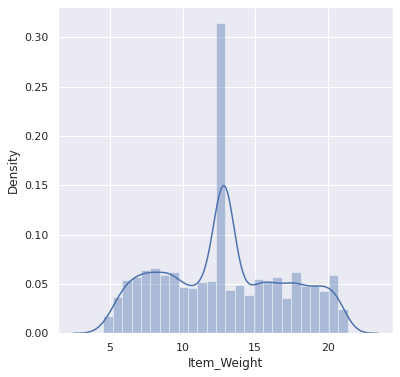

Project 12 Big Mart Sales Prediction — figure 1

ExamplePython

# Item Visibility distribution
plt.figure(figsize=(6,6))
sns.distplot(big_mart_data['Item_Visibility'])
plt.show()

Output

Output

/usr/local/lib/python3.7/dist-packages/seaborn/distributions.py:2557: FutureWarning: `distplot` is a deprecated function and will be removed in a future version
  warnings.warn(msg, FutureWarning)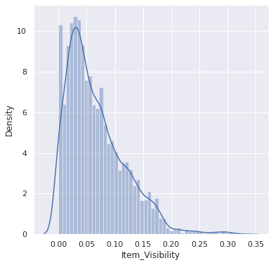

Project 12 Big Mart Sales Prediction — figure 2

ExamplePython

# Item MRP distribution
plt.figure(figsize=(6,6))
sns.distplot(big_mart_data['Item_MRP'])
plt.show()

Output

Output

/usr/local/lib/python3.7/dist-packages/seaborn/distributions.py:2557: FutureWarning: `distplot` is a deprecated function and will be removed in a future version
  warnings.warn(msg, FutureWarning)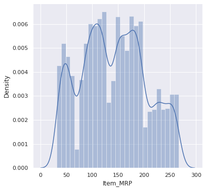

Project 12 Big Mart Sales Prediction — figure 3

ExamplePython

# Item_Outlet_Sales distribution
plt.figure(figsize=(6,6))
sns.distplot(big_mart_data['Item_Outlet_Sales'])
plt.show()

Output

Output

/usr/local/lib/python3.7/dist-packages/seaborn/distributions.py:2557: FutureWarning: `distplot` is a deprecated function and will be removed in a future version
  warnings.warn(msg, FutureWarning)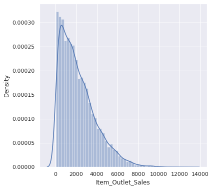

Project 12 Big Mart Sales Prediction — figure 4

ExamplePython

# Outlet_Establishment_Year column
plt.figure(figsize=(6,6))
sns.countplot(x='Outlet_Establishment_Year', data=big_mart_data)
plt.show()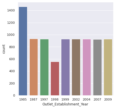

Project 12 Big Mart Sales Prediction — figure 5

Categorical Features

ExamplePython

# Item_Fat_Content column
plt.figure(figsize=(6,6))
sns.countplot(x='Item_Fat_Content', data=big_mart_data)
plt.show()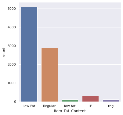

Project 12 Big Mart Sales Prediction — figure 6

ExamplePython

# Item_Type column
plt.figure(figsize=(30,6))
sns.countplot(x='Item_Type', data=big_mart_data)
plt.show()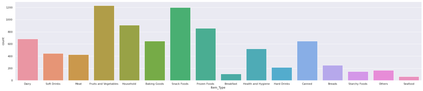

Project 12 Big Mart Sales Prediction — figure 7

ExamplePython

# Outlet_Size column
plt.figure(figsize=(6,6))
sns.countplot(x='Outlet_Size', data=big_mart_data)
plt.show()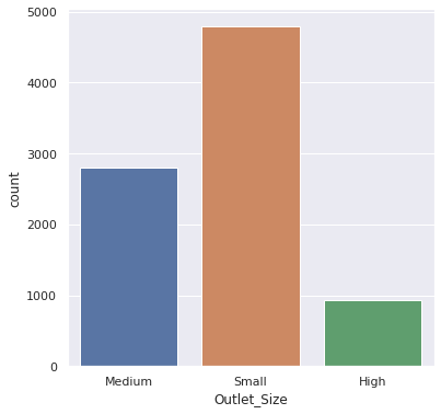

Project 12 Big Mart Sales Prediction — figure 8

Data Pre-Processing

ExamplePython

big_mart_data.head()

	Item_Identifier	Item_Weight	Item_Fat_Content	Item_Visibility	Item_Type	Item_MRP	Outlet_Identifier	…
0	FDA15	9.30	Low Fat	0.016047	Dairy	249.8092	OUT049	…
1	DRC01	5.92	Regular	0.019278	Soft Drinks	48.2692	OUT018	…
2	FDN15	17.50	Low Fat	0.016760	Meat	141.6180	OUT049	…
3	FDX07	19.20	Regular	0.000000	Fruits and Vegetables	182.0950	OUT010	…
4	NCD19	8.93	Low Fat	0.000000	Household	53.8614	OUT013	…

ExamplePython

big_mart_data['Item_Fat_Content'].value_counts()

Output

Output

Low Fat    5089
Regular    2889
LF          316
reg         117
low fat     112
Name: Item_Fat_Content, dtype: int64

ExamplePython

big_mart_data.replace({'Item_Fat_Content': {'low fat':'Low Fat','LF':'Low Fat', 'reg':'Regular'}}, inplace=True)

ExamplePython

big_mart_data['Item_Fat_Content'].value_counts()

Output

Output

Low Fat    5517
Regular    3006
Name: Item_Fat_Content, dtype: int64

Label Encoding

ExamplePython

encoder = LabelEncoder()

ExamplePython

big_mart_data['Item_Identifier'] = encoder.fit_transform(big_mart_data['Item_Identifier'])

big_mart_data['Item_Fat_Content'] = encoder.fit_transform(big_mart_data['Item_Fat_Content'])

big_mart_data['Item_Type'] = encoder.fit_transform(big_mart_data['Item_Type'])

big_mart_data['Outlet_Identifier'] = encoder.fit_transform(big_mart_data['Outlet_Identifier'])

big_mart_data['Outlet_Size'] = encoder.fit_transform(big_mart_data['Outlet_Size'])

big_mart_data['Outlet_Location_Type'] = encoder.fit_transform(big_mart_data['Outlet_Location_Type'])

big_mart_data['Outlet_Type'] = encoder.fit_transform(big_mart_data['Outlet_Type'])

ExamplePython

big_mart_data.head()

	Item_Identifier	Item_Weight	Item_Fat_Content	Item_Visibility	Item_Type	Item_MRP	Outlet_Identifier	…
0	156	9.30	0	0.016047	4	249.8092	9	…
1	8	5.92	1	0.019278	14	48.2692	3	…
2	662	17.50	0	0.016760	10	141.6180	9	…
3	1121	19.20	1	0.000000	6	182.0950	0	…
4	1297	8.93	0	0.000000	9	53.8614	1	…

Splitting features and Target

ExamplePython

X = big_mart_data.drop(columns='Item_Outlet_Sales', axis=1)
Y = big_mart_data['Item_Outlet_Sales']

ExamplePython

print(X)

Output

Output

      Item_Identifier  Item_Weight  ...  Outlet_Location_Type  Outlet_Type
0                 156        9.300  ...                     0            1
1                   8        5.920  ...                     2            2
2                 662       17.500  ...                     0            1
3                1121       19.200  ...                     2            0
4                1297        8.930  ...                     2            1
...               ...          ...  ...                   ...          ...
8518              370        6.865  ...                     2            1
8519              897        8.380  ...                     1            1
8520             1357       10.600  ...                     1            1
8521              681        7.210  ...                     2            2
8522               50       14.800  ...                     0            1

[8523 rows x 11 columns]

ExamplePython

print(Y)

Output

Output

0       3735.1380
1        443.4228
2       2097.2700
3        732.3800
4        994.7052
          ...    
8518    2778.3834
8519     549.2850
8520    1193.1136
8521    1845.5976
8522     765.6700
Name: Item_Outlet_Sales, Length: 8523, dtype: float64

Splitting the data into Training data & Testing Data

ExamplePython

X_train, X_test, Y_train, Y_test = train_test_split(X, Y, test_size=0.2, random_state=2)

ExamplePython

print(X.shape, X_train.shape, X_test.shape)

Output

Output

(8523, 11) (6818, 11) (1705, 11)

Machine Learning Model Training

XGBoost Regressor

ExamplePython

regressor = XGBRegressor()

ExamplePython

regressor.fit(X_train, Y_train)

Output

Output

[02:56:53] WARNING: /workspace/src/objective/regression_obj.cu:152: reg:linear is now deprecated in favor of reg:squarederror.

Output

Output

XGBRegressor(base_score=0.5, booster='gbtree', colsample_bylevel=1,
             colsample_bynode=1, colsample_bytree=1, gamma=0,
             importance_type='gain', learning_rate=0.1, max_delta_step=0,
             max_depth=3, min_child_weight=1, missing=None, n_estimators=100,
             n_jobs=1, nthread=None, objective='reg:linear', random_state=0,
             reg_alpha=0, reg_lambda=1, scale_pos_weight=1, seed=None,
             silent=None, subsample=1, verbosity=1)

Evaluation

ExamplePython

# prediction on training data
training_data_prediction = regressor.predict(X_train)

ExamplePython

# R squared Value
r2_train = metrics.r2_score(Y_train, training_data_prediction)

ExamplePython

print('R Squared value = ', r2_train)

Output

Output

R Squared value =  0.6364457030941357

ExamplePython

# prediction on test data
test_data_prediction = regressor.predict(X_test)

ExamplePython

# R squared Value
r2_test = metrics.r2_score(Y_test, test_data_prediction)

ExamplePython

print('R Squared value = ', r2_test)

Output

Output

R Squared value =  0.5867640914432671

Keep going: ← Lesson 47 · Lesson 49 → · Track it in the Self Guide

Finished this one?

Part of Self Guide · Stage 16: ML 4 — Evaluating & Choosing Models. Progress is saved in this browser.

Guide

Previous Next

Projects in this lesson

ML & Vision

Machine Learning Playbook & Deep Learning Lab

Interactive machine learning educational playground and hands-on laboratory covering computer vision, regression, and deep neural nets.

Project 12 Big Mart Sales Prediction

Key principles

Walkthrough

Importing the Dependencies

Data Collection and Processing

Handling Missing Values

Data Analysis

Numerical Features

Categorical Features

Data Pre-Processing

Label Encoding

Splitting features and Target

Splitting the data into Training data & Testing Data

Machine Learning Model Training

XGBoost Regressor

Evaluation

Machine Learning Playbook & Deep Learning Lab

Teaching Networking, DevOps and ML in Sinhala

Zero-Cost Hosting for InFocus SLUG 2025 — and 25 Hosting & Domain Options Compared

Life Vision: The Distributed Life